eCommix gives you the data - you decide how to look at it. Every spreadsheet it creates is a regular Google Sheet, which means all of Google Sheets' built-in tools are at your disposal. This tutorial walks through the most useful ways to tailor your view to your own workflow.
1. Use the default style or apply your own
The Style step lets you choose whether eCommix formats the sheet for you or leaves it completely unstyled so you can design it yourself.
Pick Styled for a ready-to-use layout - a green header row and alternating grey rows applied automatically after every sync. It's the fastest way to get a clean, readable sheet without any extra work.
Pick No Style if you want full control. eCommix writes only the data and never touches your formatting, so any colours, fonts, or borders you apply are preserved across every refresh. This is the best choice when you have a specific look in mind or share the sheet with a team that has its own branding.
The Include status row in header option adds a row at the top of the sheet that shows when the last sync ran and whether it succeeded or failed - useful for keeping an eye on your data without opening the app. You can disable it at any time if you'd rather keep the header clean.
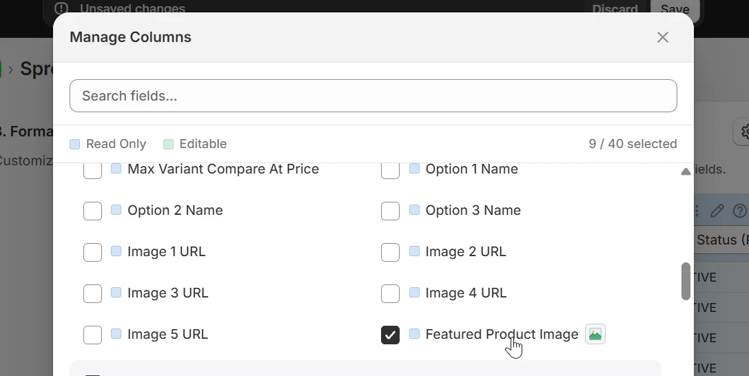
2. Select the columns you need
The Format Data step lets you choose exactly which Shopify fields appear in your spreadsheet. Click Manage Columns to check or uncheck any field, or click the pencil icon on any column header to edit it directly.
3. Reorder columns
In the Format Data step, drag any column header left or right to change the order in which columns appear in the spreadsheet.
4. Rename columns
In the Format Data step you can give any column a custom name. The rename only affects the spreadsheet header - the underlying Shopify field is unchanged.
5. Hide and show columns
Some columns are required for the sync to work - like ID fields that eCommix uses to match rows back to Shopify records - but you don't need to look at them every day. In the Format Data step you can hide any column so it stays in the sheet and eCommix can still read and write it, while keeping it out of your way.
6. Add empty columns for your own formulas
The Format Data step lets you add empty columns alongside your Shopify data columns. An empty column has no Shopify field behind it - it's a blank slot in the sheet that eCommix leaves untouched on every sync.
Use these columns for anything you need to calculate yourself: profit margins next to cost and price columns, a running total, a VLOOKUP that pulls data from another sheet, or a conditional formula that flags rows needing attention. Because eCommix never writes to those cells, your formulas are safe across every refresh.
7. Style your data
Google Sheets lets you convert any text cell into a dropdown - a coloured badge that makes categories and statuses much easier to scan at a glance. This works great for fields like Status (Product), Financial Status (Order), or Fulfillment Status (Order).
To add a dropdown, select the cells you want to convert, go to Insert → Dropdown, and choose your values and colours. From that point on, the column shows coloured dropdowns instead of plain text, and Google Sheets enforces the allowed values automatically.
Because eCommix writes only the cell values and never touches formatting or data validation rules, your dropdown configuration survives every sync refresh.
You can also add alternating row colours to make large sheets easier to read. Go to Format → Alternating colours, pick a colour scheme, and Google Sheets applies it automatically. Like dropdowns, this formatting is entirely yours - eCommix never touches it.
8. Freeze rows and columns
When your sheet has many rows or columns, it helps to keep the headers or a key identifier column always visible as you scroll. In Google Sheets, go to View → Freeze and choose how many rows or columns to lock in place.
Freezing row 1 keeps your column headers visible as you scroll down through hundreds of orders or products. Freezing the first column keeps a field like Title (Product) or Order Number in view as you scroll right through the rest of the data.
9. Add filters to focus on what matters
Google Sheets filters let you temporarily hide rows that don't match your criteria, without deleting any data. Click any header cell, then go to Data → Create a filter. A filter icon appears on every column; click it to choose which values to show or hide.
For example, you can filter an Orders sheet to show only unfulfilled orders, or a Products sheet to show only active products from a specific vendor. Use Filter views (Data → Filter views → Create new filter view) so each person on a shared sheet can have their own view without affecting anyone else.
10. Insert product images
Some fields in eCommix embed images directly into the spreadsheet cell rather than writing a URL. In Manage Columns, look for fields with the image icon - such as Featured Product Image or Featured Variant Image - and add them to your export.
Once synced, the images appear as thumbnails inside the cells. Resize the row height to make them more visible. This is especially useful for product catalogues and inventory sheets where you want a visual reference alongside the data.
The goal: your data, your workflow
eCommix is designed to give you a clean, accurate snapshot of your Shopify store in Google Sheets and then get out of the way. The underlying data refreshes on your schedule, but the presentation - styles, chips, hidden columns, frozen panes, filters, formulas, and images - is entirely yours to set up once and keep forever.